_{Prompt: Create a hyper-realistic, 4K image of a minimalist crystal glass desk with a computer on it. The computer display shows a simple, minimalist lock icon centered on the screen. The scene should include a few harmonious plants placed on or near the desk, and there should be a large window that lets in natural light. Ensure that the computer and monitor are neutral with no visible logos or branding. The aesthetic should be modern and clean, emphasizing simplicity and neutrality.}

_{Source: Generated on https://ideogram.ai/}

_{Editing: May require minor adjustments in Adobe Express (express.adobe.com)}

Introduction.      

To start this tutorial, I will answer the question that many users have asked me regarding the protection of the work done in our spreadsheets, specifically about how to develop a formula in Excel that does exactly what we want and prevents accidental deletion by users, especially when sharing the work with multiple collaborators.

There are even those who are protective of their work or, for purely professional reasons, do not want to show the formulas or how they reached this or that result. Regardless of their reasons, there is a simple way to accomplish this.

Another common situation, especially for self-learners, is when you find a workbook that has exactly the calculation you need, but you can't see the formula. In this tutorial, I'll briefly explain how to protect the sheet or, in this case, how to unprotect it when the password is known.

Protecting the Excel Sheet: Advanced Security Methods.

In the previous article Beyond Excel formulas build an effortless Quotation System [Tutorial], I concluded by discussing the importance of sheet protection, since many of us, especially Excel beginners, often struggle to achieve specific results and worry about accidental deletions. This concern extends even to experienced spreadsheet users, as various factors can affect our "inspiration" during work.

I also mentioned that while we might write formulas to verify results, even a simple sum, placing these calculations in certain cells can potentially disrupt the entire worksheet's functionality, particularly because our memory of formula locations can be unreliable.

That's why in this tutorial we're going to show you the types of protection that exist in Excel and how to implement them. To demonstrate this, I will use the archive from our previous article's exercise. We have several methods of cell protection:

Basic Methods of Protection:

· Locked: When we select locked and protect the Excel sheet, the cell can be selected or not, depending on the settings. You can view the formula but cannot delete it.

· Hidden: When we select hidden, depending on the configuration, the cell can be selected, but its contents remain invisible in the formula bar.

Additional Methods of Protection:

· Data Validation: Allows you to restrict the type of information that can be entered in a cell.

· Book-Level Protection: Offers an additional layer of security by protecting the entire structure of the workbook.

· Ranges with Permission: Allows you to assign specific permissions to different users for different cell ranges.

Cell Format Access

The Format Cells option can be accessed in the following ways:

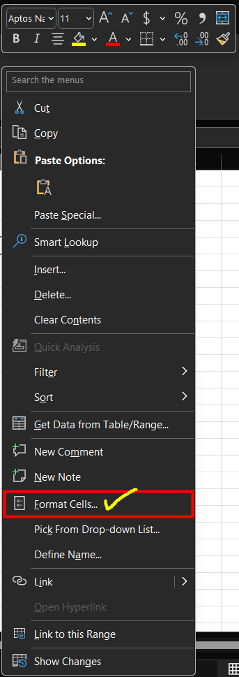
· Right-click on any cell (preferably the one or cells you want to hide).

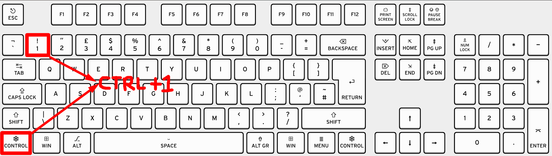
· We can use the keyboard shortcut CTRL + 1.

· We can click on the Launcher dialog box from the toolbar located in Home -> Alignment.

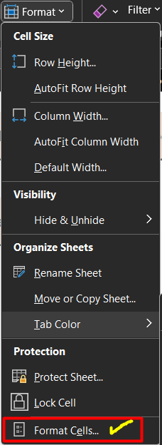
· Either Home -> Cells -> Format.

Then we just click on Format cells.

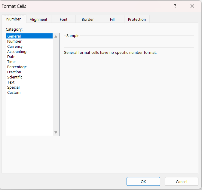
· With any of the above methods we can see the Cell Format.

Applying data protection to our Excel sheets: Step by step.

Initial Setup.

         For this exercise, we are going to apply cell protection focusing on the Locked feature. However, for this to work, we must first apply protection at the workbook level; otherwise, it won't be effective.

Similarly, to demonstrate how it works, we will apply the Hidden cell protection to see its effects. Don't worry—in this exercise, I will apply this protection only to cells containing text, and the password will simply be "Enter."

Without further delay, let's use the keyboard shortcut CTRL+1 to open Cell Format, then navigate to the Protect tab. As you can see, the Locked option is enabled by default.

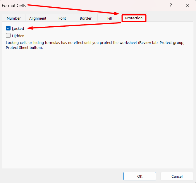
If we want to protect our sheet while still allowing users to input information, we need to deselect the Locked box for cells where data entry is required.

· In the Quotation sheet select the following Cells:

- B9

- B13

- B15

- D14

- F6

- F7

- F10

 We will disable the locked box.

· For demonstration purposes, we will select the range B5:B7 from our Quotation sheet and apply the Hidden protection. I pick this range because doesn’t have any formula and if you want to use this spreadsheet you won’t have any worries to use it.

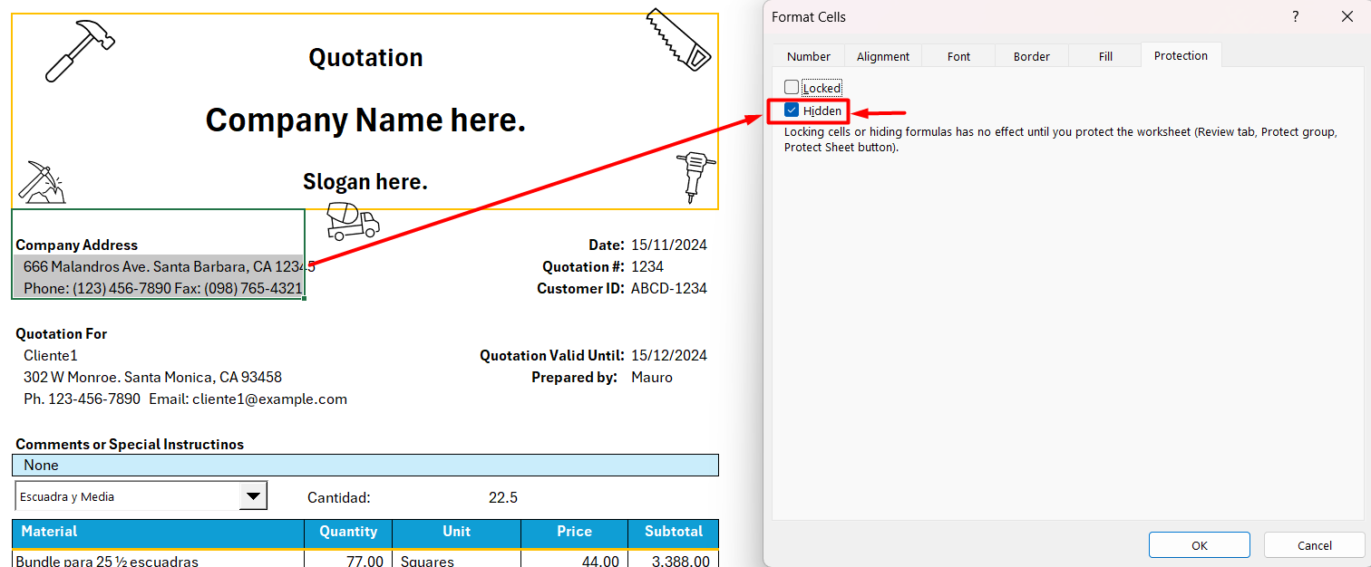
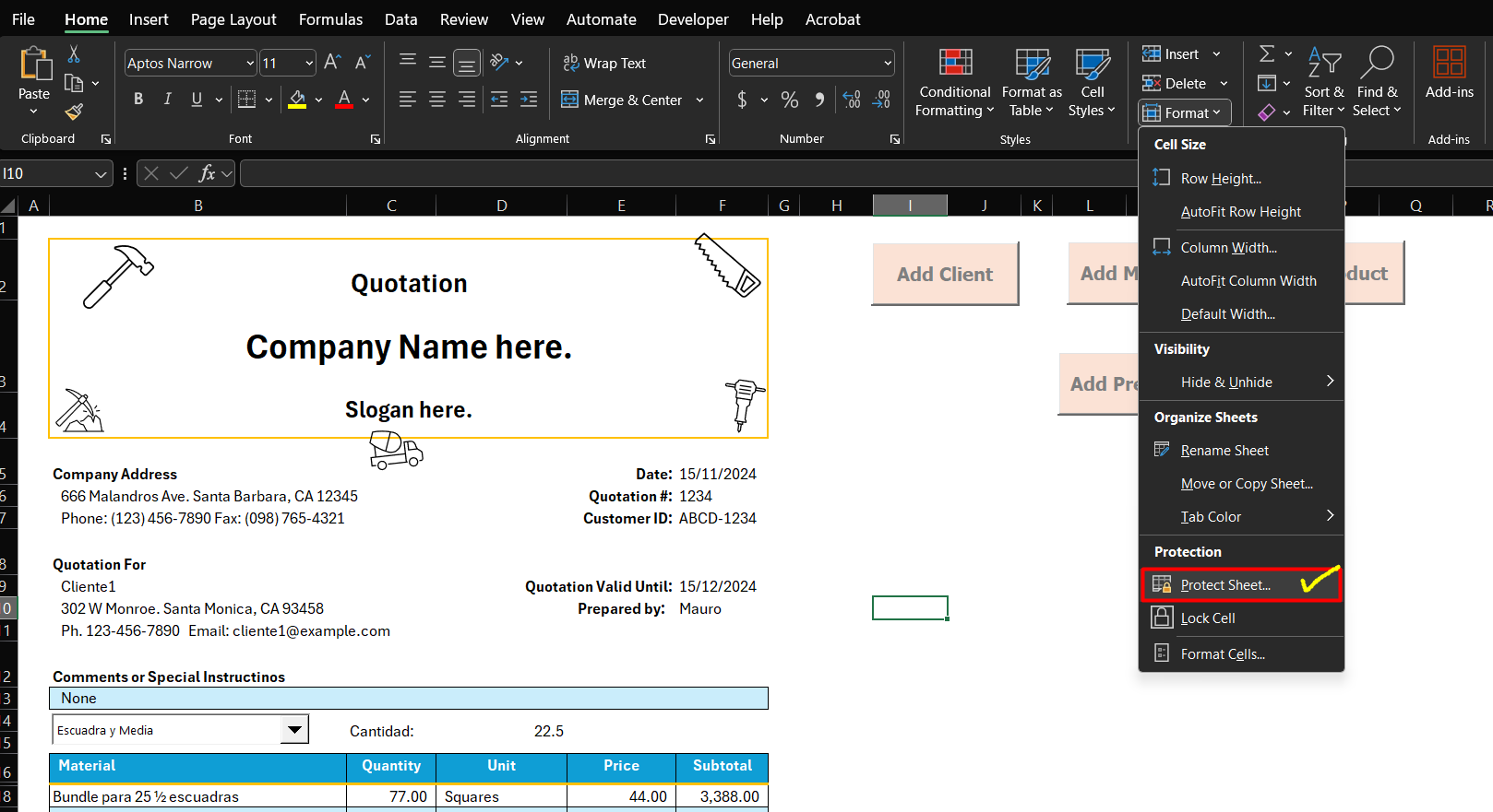
·      To see how this works, navigate to Home -> Cells -> Format.

Then select Protect Sheet...

Configuring Protection.

· This will display the Protect Sheet menu.

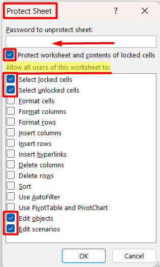
-       The dialog asks for a Password to unprotect the sheet. You can leave this blank to allow users to unprotect it later, or set a password that best suits your needs.

-       By default, the Protect sheet and contents of locked cells checkbox are selected. We'll keep this setting.

-       Under Allow Users of this spreadsheet, the default options Select locked cells and Select unlocked cells are typically enabled. This relates to what we discussed in Basic Methods of Protection regarding cell selection permissions.

-       Below Allow users in this sheet, you'll find various permission levels you can grant to users. The complete list of permissions includes:

o  Select Locked Cells: Allows the user to select, but not modify, protected cells.

o  Select unlocked cells: Allows you to select and modify cells that are not protected.

o  Cell Formatting: Enables changes to visual formatting (color, font, borders, etc.)

o  Column formatting: Allows you to modify the width and general formatting of columns.

o  Row Formatting: Enables changes to the overall height and formatting of rows.

o  Insert Columns: Allows you to add new columns in the sheet.

o  Insert Rows: Allows you to insert new rows.

o  Insert Hyperlinks: Enables link creation within the sheet.

o  Delete columns: Allows you to delete entire columns.

o  Delete rows: Enables deletion of entire rows.

o  Sort: Allows you to rearrange data in ascending or descending order.

o  Use automatic filters: Enables the use of filters to analyze data.

o  Use PivotTables: Allows you to create and modify existing PivotTables.

o  Edit Objects: Allows you to modify graphics, shapes, images, and other inserted objects.

o  Edit Scenarios: Enables modification of scenarios if they exist in the sheet.

It is important to carefully select these permissions based on the access level you want to grant your users. For example, when creating a data entry template, you might enable only Select Unlocked Cells and Use Auto Filters, while keeping the rest of the sheet protected to maintain the integrity of your formulas and structure.

Note. When using Macros to update our quotation, it's crucial to properly unlock and lock the sheet to avoid issues. Follow these steps:

· Open the VBA Editor ALT + F11.

· Around line of code 10 after the code:

Set ws = ThisWorkbook.Sheets("Quotation")

Then add:

add: ws.Unprotect ""

You can type any password between quotations you would like.

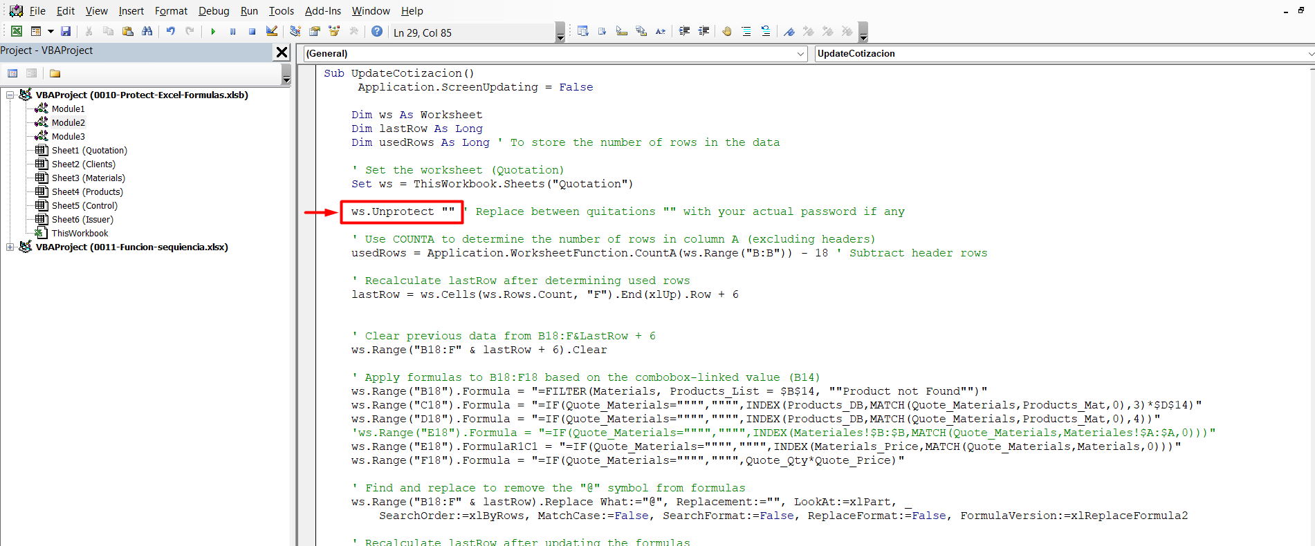
We add this unprotect line to allow Excel to modify content when updating the quotation.

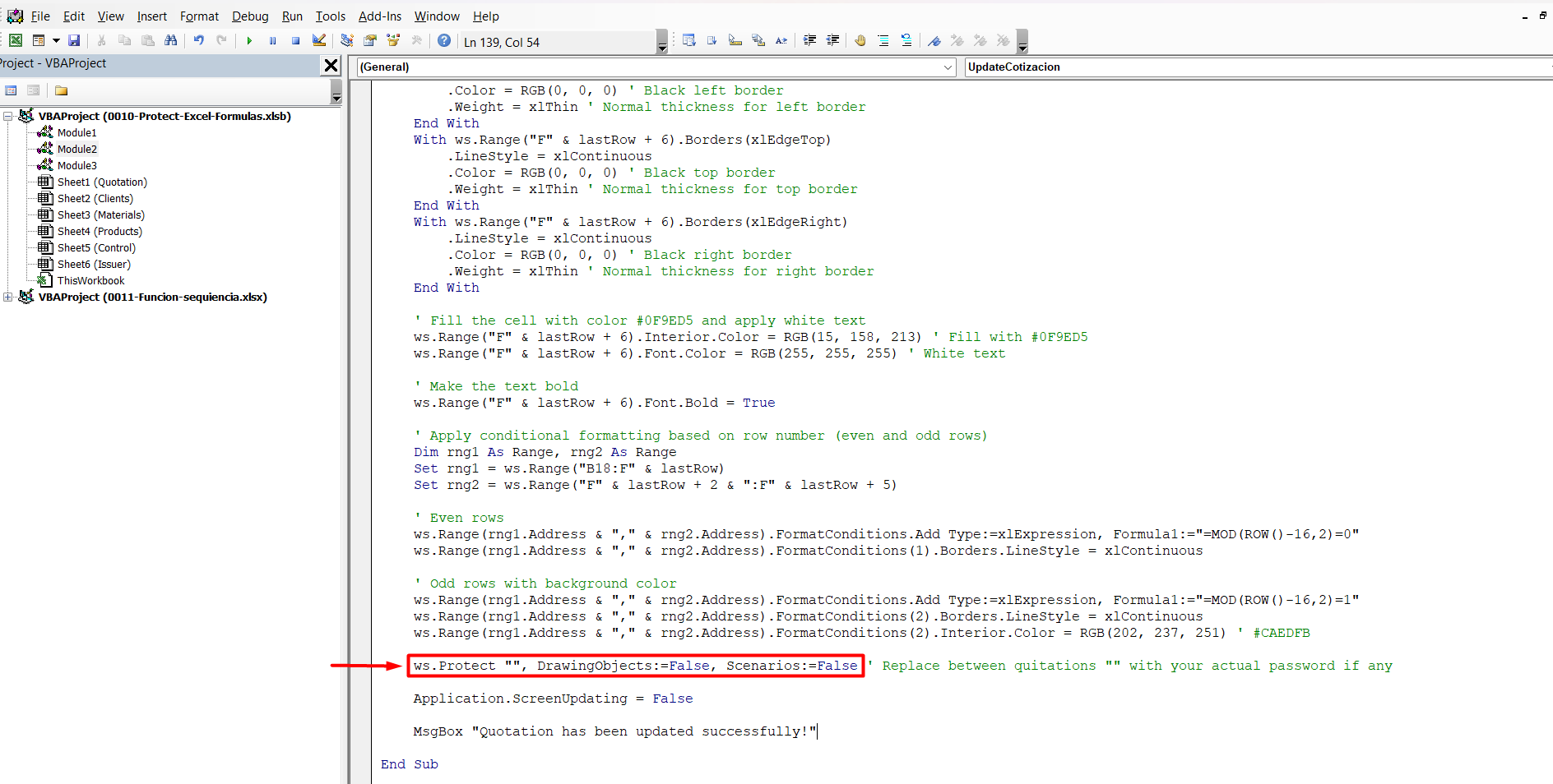
· A Before closing the workbook, ensure you reapply protection in the antepenultimate line of code

Application.ScreenUpdating = False

Then add:

ws.Protect "", DrawingObjects:=False, Scenarios:=False

Breakdown of the protection settings:

- Protect “” : Enter your desired password (left blank for practical purposes).

- DrawingObjects:=False: Enables manipulation of form controls

- Scenarios:=False: Allows seamless quotation modifications

Cell Protection Verification and Results in Excel: Practical Tests.

         To see the results of cell protection, let's see how our Quotation sheet where we will perform the following tests to confirm functionality:

Functionality Testing:

1. In cell B9, we changed the client. As you can see (and no screenshot is necessary here), it behaves normally no errors or messages. The same behavior occurs in cell B13, D14, F6, F7 as well as F10, confirming that the unlocked cells are working correctly.
2. Now, in the cells of Range B16:F21, let's try to modify some data. What happens? Did you get a screen like the one below?

As we can see, the cell or graph is protected, so if we want to make any changes, it's necessary to unprotect the sheet. This is the expected behavior for locked cells.

1. Let's try any of the ranges (B5:B7) where we selected that we wanted the information in the cell to be hidden.

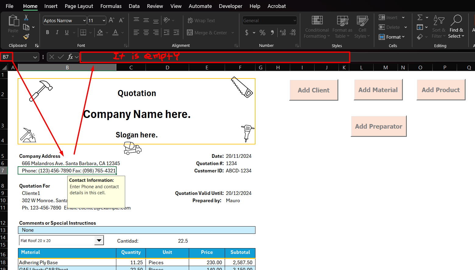
As we can see in the formula bar, it appears empty. This isn't because there's no value, but rather because it's Hidden, thus complying with our configuration.

Practical Implementation and Recommendations:

We can see how simple and practical it is to protect your workbooks and cells containing formulas. We can not only hide but also block content to protect our work, ensuring the correct functioning of our workbook and/or electronic worksheets, their integrity, and avoiding human errors.

Conclusions.

         As we have seen, the procedure to protect our cells and workbooks in Excel is straightforward and easy to execute. However, let's be honest—it's not the most secure or comprehensive method available. While many people often refer to Excel as a "database" due to its ability to store information in tables, it technically isn't one. If you're handling sensitive information or require a true data management system with robust security, you should consider migrating to a more professional solution like SQL.

That said, for protecting work from human error or everyday accidents, Excel fully meets our objectives. We can easily add a basic layer of security to our spreadsheets that serves most common needs.

Would you like to learn more about other protection methods in Excel? We can explore the additional protection methods mentioned earlier in future articles. Meanwhile, you can download the protected exercise file using the following link to practice and see the final results for yourself.

Excel is an exceptionally good instrument; nonetheless, as the technology develops, it is also turning out to become a much more flexible platform. If you want to be at the forefront of new trends and advancements in your field, if you want to be more productive, and if you want to meet your goals earlier, then two possibilities might be intriguing to you:

·      This is ideal for users with a desire to every time have the tools with the newest features and continuous updates Microsoft 365

·      It is more suitable for use by experts who prefer to have, an all-in-one, long-term solution (one-time purchase): Office 2021 Perpetual License

No matter which alternative you choose, both of them can unleash you with a bunch of tools that can convert your workflows and also pull some new doors to success. By far, I want you to go for the option that best supports your ambitions and the way you are most comfortable with working. Here is the link of today’s excercice.

Was this tutorial helpful? Don't forget to share it and leave your feedback on what other Excel topics you'd like us to explore.